Researchers and data‑driven teams frequently turn to Google Sheets for rapid analysis, yet many miss the powerful variations of the INDEX MATCH combo that can replace clunky VLOOKUPs, reduce errors, and keep worksheets scalable. This article dissects typical mistakes—such as static range references and mismatched data types—and presents smarter alternatives that let users truly unlock hidden index match functions in Google Sheets.
Scenario 1: A rotating inventory list that breaks every month
Why the classic INDEX MATCH fails
- Hard‑coded column numbers (e.g.,
=INDEX(B:B, MATCH(D2, A:A, 0))) become obsolete when columns are reordered. - Implicit intersections ignore hidden rows, returning the wrong item when filters are applied.
Smarter approach: Dynamic column lookup
Combine MATCH with INDEX on FILTER to locate both the row and the correct column regardless of reordering:
- Identify the target column:
=MATCH("Price", 1:1, 0). - Retrieve the value:
=INDEX(FILTER(A2:Z, A2:A = D2), , MATCH("Price", 1:1, 0)).
This method automatically follows any column move, erasing the need for manual updates.
Scenario 2: Cross‑sheet lookups that return #N/A on missing data
Typical mistake: Ignoring error handling
When a lookup fails, plain INDEX(MATCH(...)) propagates #N/A, breaking downstream calculations.
Alternative: IFERROR wrapped with ARRAYFORMULA
Wrap the lookup in IFERROR and expand it with ARRAYFORMULA to supply a default value across an entire column:
=ARRAYFORMULA(IFERROR(INDEX(ImportRange("sheet_key","Data!A:Z"),
 MATCH(A2:A, ImportRange("sheet_key","Data!A:A"), 0), 3), "Not found"))
This keeps reports clean and highlights only truly missing records.
Scenario 3: Multi‑criteria searches that require more than a single key
Common error: Stacking MATCH functions
Attempting MATCH on concatenated keys (e.g., A2&B2) often leads to mismatched data types and hidden spaces.
Preferred solution: Use FILTER with INDEX
Leverage FILTER to handle multiple conditions directly, then apply INDEX on the filtered result:
=INDEX(FILTER(Data!C:C, Data!A:A = D2, Data!B:B = E2), 1)Because FILTER respects all criteria simultaneously, it eliminates the fragile concatenation step.
Scenario 4: Large datasets where performance degrades
Problem: Repeated volatile functions
Every time a sheet recalculates, full‑range INDEX(MATCH) formulas scan thousands of rows, causing noticeable lag.
Optimization: Use helper columns and QUERY
Store the row identifier in a hidden helper column, then query that column once:
- Create a helper:
=ROW()in column Z. - Run a single
QUERY:=QUERY(Data!A:Z, Z:Z, "select Col3 where Col1 = '"&D2&"' limit 1", 0).
The QUERY engine is optimized for large tables, dramatically reducing recalculation time.
Implications for research workflows
By moving beyond the textbook INDEX MATCH pattern, analysts gain three tangible benefits: resilience against structural changes, clarity when handling missing data, and speed on expansive datasets. The hidden variations highlighted here encourage a shift from “quick‑and‑dirty” lookups to robust, maintainable formulas—an essential upgrade for any detail‑oriented researcher who relies on Google Sheets for reproducible analysis.
کتاب جدول مندلیف عناصر شیمیایی در سایز A5 اندیشه جم

کتاب جدول مندلیف عناصر شیمیایی در سایز A5 اندیشه جم
جدول مندلیف فارسی (جدول تناوبی عناصر) | آموزش کامل ۲۰۲۵ - خرید مواد شیمیایی

جدول مندلیف فارسی (جدول تناوبی عناصر) | آموزش کامل ۲۰۲۵ - خرید مواد شیمیایی
خرید و قیمت جدول مندلیف A3 (جدول تناوبی عناصر پرس شده دوطرفه-فارسی و
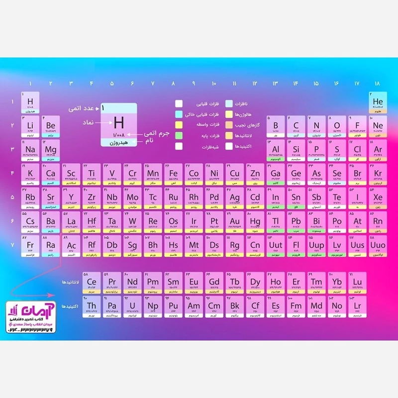
خرید و قیمت جدول مندلیف A3 (جدول تناوبی عناصر پرس شده دوطرفه-فارسی و ...
قیمت و خرید پوستر آموزشی طرح جدول تناوبی عناصر مندلیف مدل جیبی کد 10
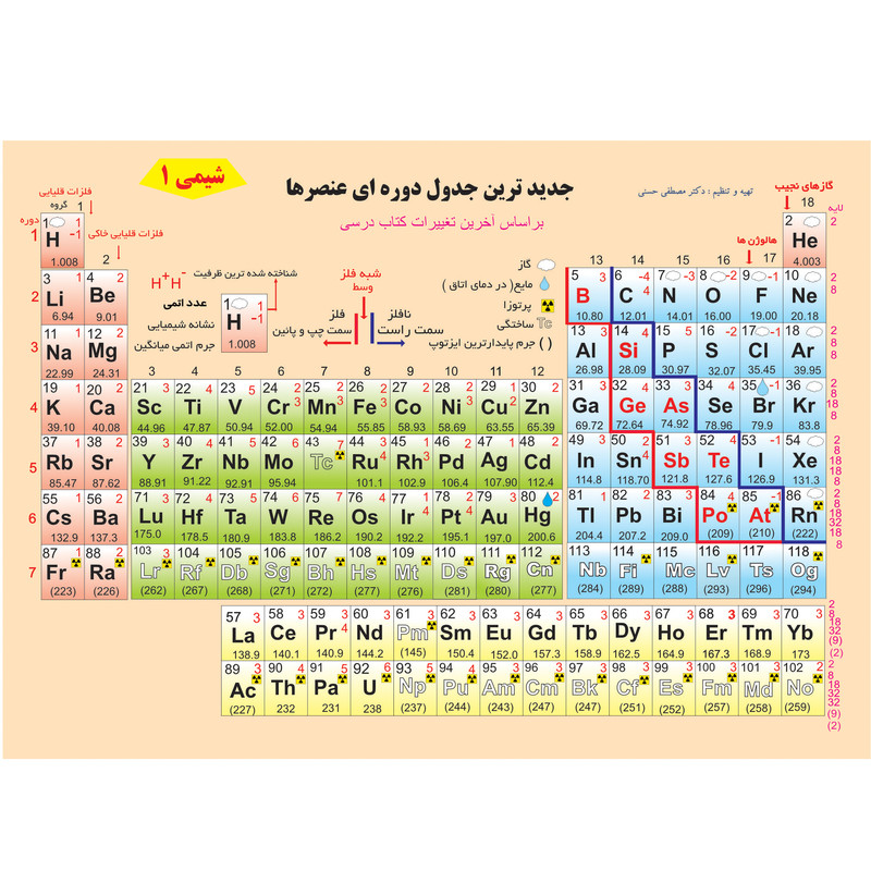
قیمت و خرید پوستر آموزشی طرح جدول تناوبی عناصر مندلیف مدل جیبی کد 10
خرید پوستر آموزشی جدول تناوبی عناصر مندلیف سایز A3
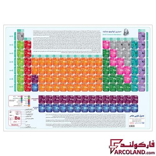
خرید پوستر آموزشی جدول تناوبی عناصر مندلیف سایز A3